How the ABC algorithm works in ABCoptim

library(ABCoptim)

The Artificial Bee Colony (ABC) algorithm is a population-based optimization method inspired by the way honey bees explore and exploit food sources. In ABCoptim, each candidate solution is a food source, better solutions get more attention from the colony, and poorly performing solutions are eventually replaced. The package implements the minimization version described by Karaboga (2005), with both R and C++ backends.

Step by step

The abc_optim() implementation follows the same sequence on every cycle:

1. Initialize food sources. The code creates FoodNumber candidate solutions inside the bounds lb and ub. In abc_optim(), the first population is placed on an evenly spaced grid using seq() for each parameter.
2. Evaluate and score them. The objective function is evaluated at every food source and converted into a fitness value. Smaller objective values imply better fitness.
3. Employed bee phase. Each food source proposes a one-coordinate mutation using the difference between itself and a randomly chosen neighbor. If the new point improves fitness, it replaces the old one.
4. Onlooker bee phase. Food sources with larger fitness receive more attention. abc_optim() computes probabilities from relative fitness and lets onlookers update promising sources using the same greedy replacement rule.
5. Memorize the best source. After the onlooker phase, the algorithm stores the best solution found so far and records it in the optimization history.
6. Stop if the best value has not improved enough. The object keeps a persistence counter and stops when the best value remains unchanged for more than criter cycles, or when maxCycle is reached.
7. Scout bee phase. If a food source has been tried at least limit times without improvement, the source with the largest trial counter is reinitialized.

Two implementation details are worth keeping in mind when using the package:

• The objective function must always return a single finite numeric value.
• Bounds are enforced after each mutation, so proposed values outside [lb, ub] are clipped back to the boundary.

Example: minimizing the Booth function

The package examples already cover the cosine benchmark, a one-dimensional function, a sphere, and an OLS problem. The next example uses the two-dimensional Booth function,

$$f(x, y) = (x + 2y - 7)^2 + (2x + y - 5)^2,$$

which has its global minimum at $(1, 3)$.

booth <- function(x) {
  (x[1] + 2 * x[2] - 7)^2 + (2 * x[1] + x[2] - 5)^2
}

set.seed(2026)
ans <- abc_optim(
  par = c(0, 0),
  fn = booth,
  lb = -10,
  ub = 10,
  FoodNumber = 20,
  limit = 40,
  criter = 75,
  maxCycle = 500
)

ans[c("par", "value", "counts")]

$par
[1] 1 3

$value
[1] 3.204614e-16

$counts
function
     461 

The estimated optimum should be close to (1, 3), and the objective value should be near zero.

plot(ans)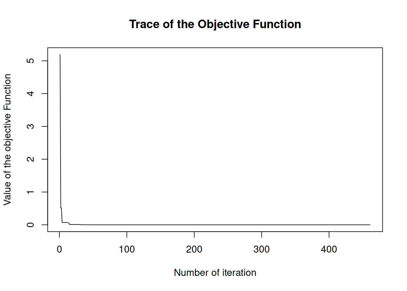

This plot shows the best point found at each cycle. In practice, that trace is useful for checking whether the colony is still improving or whether criter, limit, or FoodNumber should be adjusted.