Skip to contents

Imaginary Network Motifs: Analyzing Systematic Perception Errors

Understanding how people perceive social networks reveals systematic biases in human cognition. This vignette demonstrates the imaginary network motifs framework using the classic Krackhardt dataset to identify when perceived network patterns deviate significantly from chance expectations.

Setup

library(imaginarycss)
library(ggplot2)
library(dplyr)
library(reshape2)

# Load Krackhardt high-tech managers data
data(krack_advice)
data(krack_friendship) 
data(Krack_friendship_perceptions)
Warning in data(Krack_friendship_perceptions): data set
'Krack_friendship_perceptions' not found
data(Krack_advice_perceptions)
Warning in data(Krack_advice_perceptions): data set 'Krack_advice_perceptions'
not found
# Convert to adjacency matrices
advice_matrix <- acast(krack_advice, from ~ to, value.var = "value", fill = 0)
friendship_matrix <- acast(krack_friendship, from ~ to, value.var = "value", fill = 0)

Data Overview

cat("Dataset: 21 managers in a high-tech company\n")
Dataset: 21 managers in a high-tech company
cat("Friendship network - Edges:", sum(friendship_matrix), 
    "| Density:", round(sum(friendship_matrix)/(21*20), 3), "\n")
Friendship network - Edges: 102 | Density: 0.243 
cat("Advice network - Edges:", sum(advice_matrix), 
    "| Density:", round(sum(advice_matrix)/(21*20), 3), "\n")
Advice network - Edges: 190 | Density: 0.452 
cat("Perception networks per type:", length(krack_friendship_perceptions))
Perception networks per type: 21

Creating Network Graphs

# Combine true networks with individual perceptions
friendship_graph <- new_barry_graph(c(list(friendship_matrix), krack_friendship_perceptions))
advice_graph <- new_barry_graph(c(list(advice_matrix), krack_advice_perceptions))

Observed Motif Patterns

# Count imaginary census motifs
friendship_observed <- count_imaginary_census(friendship_graph)
advice_observed <- count_imaginary_census(advice_graph)

# Clean and aggregate motif data
process_motifs <- function(census_data) {
  census_data %>%
    mutate(motif_type = gsub("\\([0-9]+\\)$", "", name)) %>%
    group_by(motif_type) %>%
    summarise(
      total = sum(value),
      mean_per_person = mean(value),
      variation = var(value),
      .groups = 'drop'
    ) %>%
    arrange(desc(total))
}

friendship_summary <- process_motifs(friendship_observed)
advice_summary <- process_motifs(advice_observed)

# Show top patterns
cat("Top friendship motifs:\n")
Top friendship motifs:
print(head(friendship_summary[, 1:3], 6))
# A tibble: 6 × 3
  motif_type                             total mean_per_person
  <chr>                                  <dbl>           <dbl>
1 "(01) Accurate null "                   2472          118.
2 "(05) Accurate assym "                   529           25.2
3 "(07) Partial false positive (assym) "   378           18
4 "(02) Partial false positive (null) "    276           13.1
5 "(10) Accurate full "                    269           12.8
6 "(09) Partial false negative (full) "    181            8.62
cat("\nTop advice motifs:\n")

Top advice motifs:
print(head(advice_summary[, 1:3], 6))
# A tibble: 6 × 3
  motif_type                             total mean_per_person
  <chr>                                  <dbl>           <dbl>
1 "(05) Accurate assym "                  1052            50.1
2 "(01) Accurate null "                    992            47.2
3 "(10) Accurate full "                    469            22.3
4 "(04) Partial false negative (assym) "   463            22.0
5 "(07) Partial false positive (assym) "   412            19.6
6 "(09) Partial false negative (full) "    395            18.8

Distribution Visualization

# Create distribution plot
create_distribution_plot <- function(census_data, network_name) {
  census_clean <- census_data %>%
    mutate(motif_type = gsub("\\([0-9]+\\)$", "", name))
  
  ggplot(census_clean, aes(x = value)) +
    geom_histogram(bins = 8, fill = "steelblue", alpha = 0.7, color = "white") +
    facet_wrap(~motif_type, scales = "free", labeller = label_wrap_gen(width = 20)) +
    labs(title = paste("Distribution of Motif Types -", network_name),
         subtitle = "Individual-level counts across 21 managers",
         x = "Count", y = "Frequency") +
    theme_minimal() +
    theme(
      strip.text = element_text(size = 9, face = "bold"),
      plot.title = element_text(size = 14, face = "bold"),
      axis.text = element_text(size = 8)
    )
}

# Plot distributions
friendship_dist_plot <- create_distribution_plot(friendship_observed, "Friendship")
print(friendship_dist_plot)

Null Model Testing

# Generate null distributions via CSS sampling
cat("Generating null models (100 samples each)...\n")
Generating null models (100 samples each)...
set.seed(331)
friendship_null <- replicate(100, {
  count_imaginary_census(new_barry_graph(sample_css_network(friendship_graph)))
}, simplify = FALSE)

advice_null <- replicate(100, {
  count_imaginary_census(new_barry_graph(sample_css_network(advice_graph)))
}, simplify = FALSE)

Statistical Significance Analysis

# Calculate Z-scores against null expectation
test_significance <- function(observed, null_samples) {
  # Aggregate observed by motif type
  obs_agg <- observed %>%
    mutate(motif = gsub("\\([0-9]+\\)$", "", name)) %>%
    group_by(motif) %>%
    summarise(observed = sum(value), .groups = 'drop')
  
  # Process null samples 
  null_matrix <- sapply(null_samples, function(x) {
    x %>% 
      mutate(motif = gsub("\\([0-9]+\\)$", "", name)) %>%
      group_by(motif) %>%
      summarise(null_val = sum(value), .groups = 'drop') %>%
      arrange(motif) %>%
      pull(null_val)
  })
  
  # Statistical testing
  obs_agg %>%
    mutate(
      null_mean = rowMeans(null_matrix),
      null_sd = apply(null_matrix, 1, sd),
      z_score = (observed - null_mean) / null_sd,
      p_value = 2 * pmin(
        rowMeans(null_matrix <= observed),
        rowMeans(null_matrix >= observed)
      ),
      significant = abs(z_score) > 1.96 & p_value < 0.05,
      direction = ifelse(z_score > 0, "Elevated", "Reduced")
    ) %>%
    arrange(desc(abs(z_score)))
}

# Run tests
friendship_results <- test_significance(friendship_observed, friendship_null)
advice_results <- test_significance(advice_observed, advice_null)

Key Findings

# Display significant results
cat("=== SIGNIFICANT DEVIATIONS FROM CHANCE ===\n\n")
=== SIGNIFICANT DEVIATIONS FROM CHANCE ===
show_significant <- function(results, network_name) {
  sig_results <- results[results$significant, ]
  if(nrow(sig_results) > 0) {
    cat(network_name, "Network:\n")
    print(sig_results[, c("motif", "observed", "z_score", "p_value", "direction")])
    cat("\n")
  } else {
    cat(network_name, "Network: No significant deviations\n\n")
  }
}

show_significant(friendship_results, "Friendship")
Friendship Network:
# A tibble: 7 × 5
  motif                                  observed z_score p_value direction
  <chr>                                     <dbl>   <dbl>   <dbl> <chr>
1 "(07) Partial false positive (assym) "      378   26.9        0 Elevated
2 "(05) Accurate assym "                      529  -15.6        0 Reduced
3 "(01) Accurate null "                      2472   14.6        0 Elevated
4 "(02) Partial false positive (null) "       276  -13.6        0 Reduced
5 "(06) Mixed assym "                          98   13.3        0 Elevated
6 "(04) Partial false negative (assym) "      171   -5.64       0 Reduced
7 "(03) Complete false positive (null) "        3   -5.36       0 Reduced  
show_significant(advice_results, "Advice")
Advice Network:
# A tibble: 6 × 5
  motif                                  observed z_score p_value direction
  <chr>                                     <dbl>   <dbl>   <dbl> <chr>
1 "(07) Partial false positive (assym) "      412    7.87       0 Elevated
2 "(01) Accurate null "                       992    7.38       0 Elevated
3 "(02) Partial false positive (null) "       343   -6.12       0 Reduced
4 "(05) Accurate assym "                     1052   -5.33       0 Reduced
5 "(06) Mixed assym "                         173    3.59       0 Elevated
6 "(03) Complete false positive (null) "       30   -3.58       0 Reduced  
# Visualization
top_n <- 8
combined <- rbind(
  data.frame(friendship_results[1:top_n, ], Network = "Friendship"),
  data.frame(advice_results[1:top_n, ], Network = "Advice")
)

significance_plot <- ggplot(combined, aes(x = reorder(motif, z_score), y = z_score)) +
  geom_col(aes(fill = significant), alpha = 0.8, width = 0.7) +
  geom_hline(yintercept = c(-1.96, 1.96), linetype = "dashed", 
             color = "red", alpha = 0.8, size = 0.8) +
  geom_hline(yintercept = 0, color = "black", alpha = 0.4) +
  facet_wrap(~Network, scales = "free", ncol = 1) +
  coord_flip() +
  scale_fill_manual(
    values = c("FALSE" = "lightgray", "TRUE" = "steelblue"),
    name = "Significant\n(p < 0.05)"
  ) +
  labs(
    title = "Motif Significance Analysis",
    subtitle = "Z-scores vs null model | Red lines = significance threshold (±1.96)",
    x = "Motif Type",
    y = "Z-Score"
  ) +
  theme_minimal() +
  theme(
    plot.title = element_text(size = 16, face = "bold"),
    plot.subtitle = element_text(size = 12),
    axis.text.y = element_text(size = 10),
    strip.text = element_text(size = 12, face = "bold"),
    legend.position = "bottom"
  )
Warning: Using `size` aesthetic for lines was deprecated in ggplot2 3.4.0.
ℹ Please use `linewidth` instead.
print(significance_plot)

Interpretation

# Summary statistics
friend_sig_count <- sum(friendship_results$significant)
advice_sig_count <- sum(advice_results$significant)
friend_elevated <- sum(friendship_results$significant & friendship_results$z_score > 0)
advice_elevated <- sum(advice_results$significant & advice_results$z_score > 0)

cat("=== SUMMARY ===\n")
=== SUMMARY ===
cat("Friendship network:", friend_sig_count, "significant motifs (", 
    friend_elevated, "elevated,", friend_sig_count - friend_elevated, "reduced)\n")
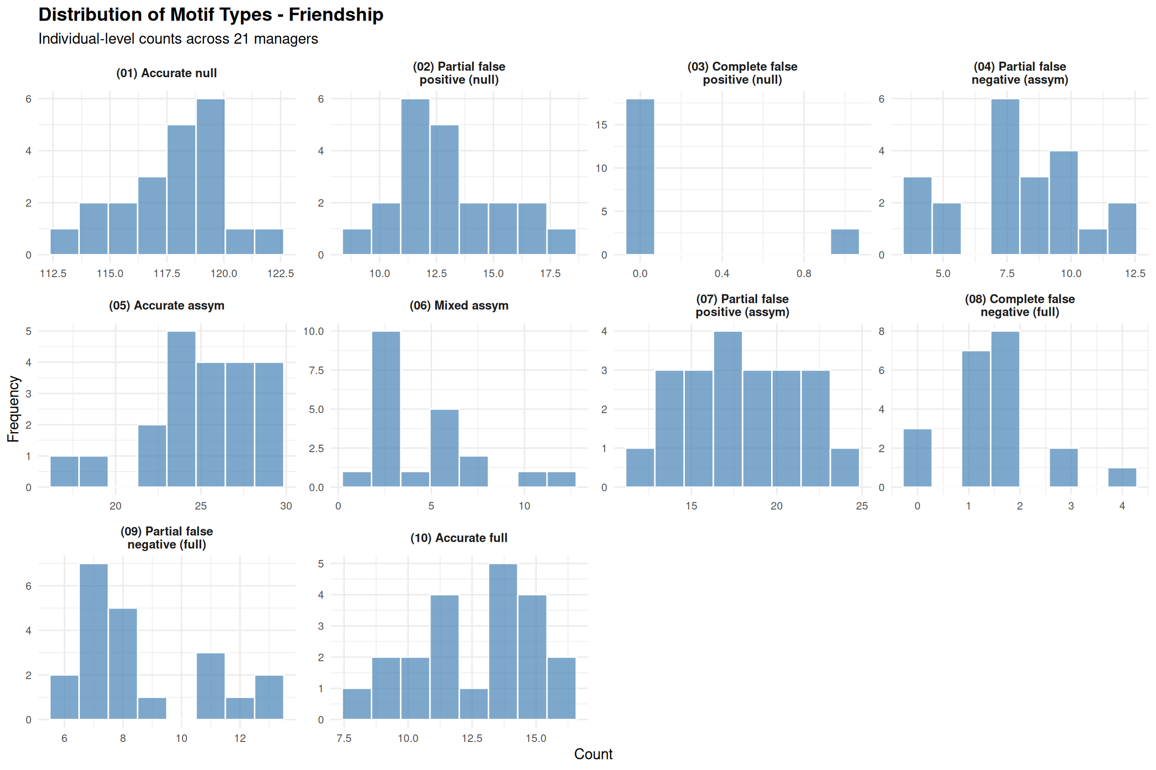
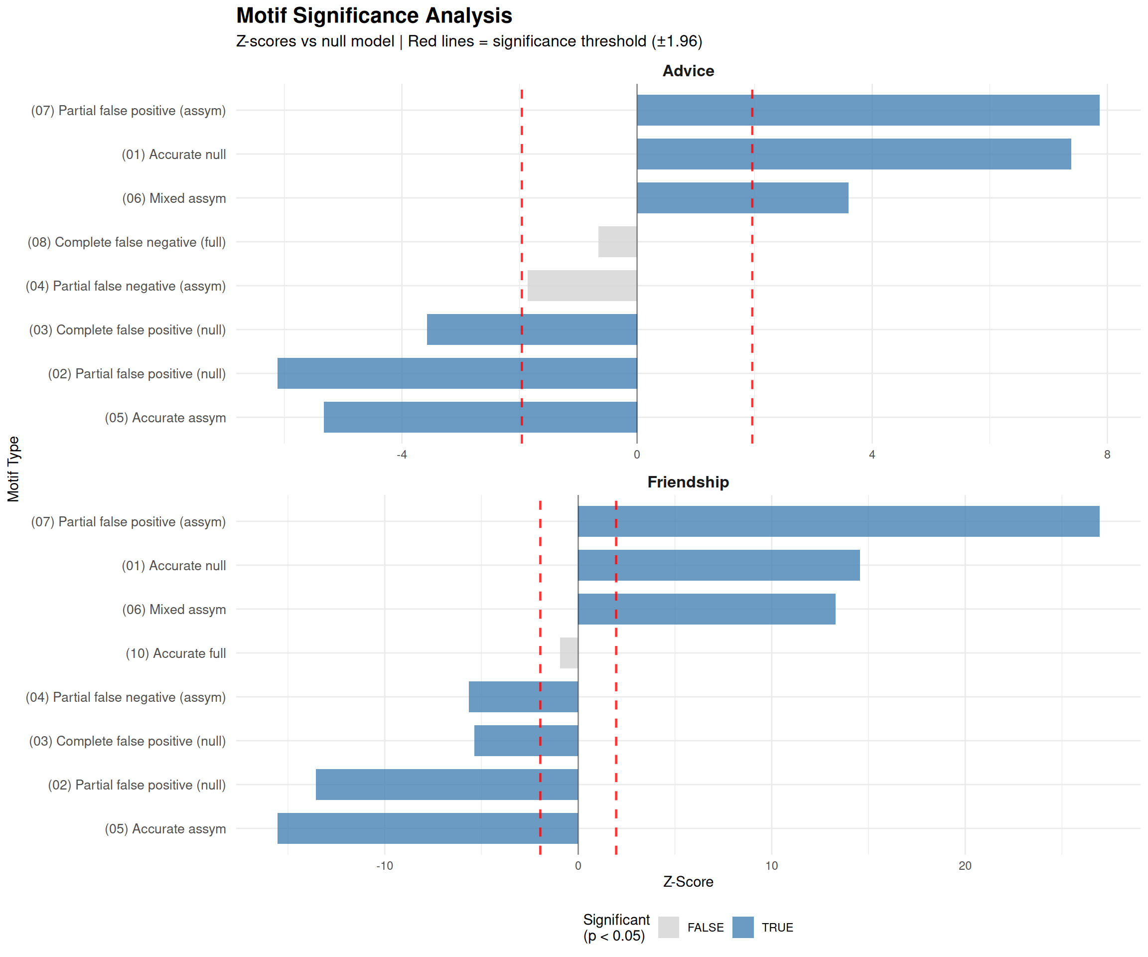
Friendship network: 7 significant motifs ( 3 elevated, 4 reduced)
cat("Advice network:", advice_sig_count, "significant motifs (",
    advice_elevated, "elevated,", advice_sig_count - advice_elevated, "reduced)\n")
Advice network: 6 significant motifs ( 3 elevated, 3 reduced)
# Effect sizes
cat("\nEffect sizes (mean |Z-score|):\n")

Effect sizes (mean |Z-score|):
cat("Friendship:", round(mean(abs(friendship_results$z_score)), 2), "\n")
Friendship: 9.71 
cat("Advice:", round(mean(abs(advice_results$z_score)), 2), "\n")
Advice: 3.67 
# Theoretical implications
cat("\n=== THEORETICAL IMPLICATIONS ===\n")

=== THEORETICAL IMPLICATIONS ===
if(friend_sig_count > advice_sig_count) {
  cat("• Friendship networks show stronger systematic biases\n")
  cat("• Consistent with balance schema and reciprocity assumptions\n")
} else {
  cat("• Advice networks show stronger systematic biases\n")
  cat("• May reflect hierarchy and expertise perception patterns\n")
}
• Friendship networks show stronger systematic biases
• Consistent with balance schema and reciprocity assumptions
cat("• Individual perception varies significantly from random baselines\n")
• Individual perception varies significantly from random baselines
cat("• Cognitive schemas systematically distort network perception\n")
• Cognitive schemas systematically distort network perception

Tie-Level Accuracy

# Individual accuracy analysis
friendship_acc <- tie_level_accuracy(friendship_graph)
advice_acc <- tie_level_accuracy(advice_graph)

# Quick comparison
acc_summary <- data.frame(
  Network = c("Friendship", "Advice"),
  True_Positive_Rate = c(mean(friendship_acc$p_1_ego, na.rm=T), 
                        mean(advice_acc$p_1_ego, na.rm=T)),
  True_Negative_Rate = c(mean(friendship_acc$p_0_ego, na.rm=T),
                        mean(advice_acc$p_0_ego, na.rm=T))
)

cat("Individual-level accuracy:\n")
Individual-level accuracy:
print(acc_summary)
     Network True_Positive_Rate True_Negative_Rate
1 Friendship          0.7501383          0.8863365
2     Advice          0.6945163          0.7948616

Conclusion

This analysis demonstrates how the imaginary network motifs framework reveals systematic biases in social network perception. By comparing observed patterns against null models generated via sample_css_network(), we identify which cognitive errors occur beyond chance expectations.

Key methodological advances:

  • Null model rigor: Random network comparison provides statistical baseline

  • Individual variation: Framework captures person-level differences in perception accuracy

  • Motif-level analysis: Goes beyond simple accuracy to examine structural error patterns

  • Systematic bias detection: Identifies cognitive schemas that distort network perception

The results illuminate how human cognition systematically misperceives social structure, with implications for organizational behavior, social psychology, and network analysis methodology.