Analyzing Perceptual Errors and Individual Accuracy

Sima Najafzadehkhoei

2025-12-12

library(imaginarycss)
library(ggplot2)
library(dplyr)

Attaching package: 'dplyr'

The following objects are masked from 'package:stats':

    filter, lag

The following objects are masked from 'package:base':

    intersect, setdiff, setequal, union

library(viridis)

Loading required package: viridisLite

# Theme and colors
theme_set(theme_minimal(base_size = 12) +
  theme(plot.title = element_text(size = 16, face = "bold", color = "#2c3e50"),
        plot.subtitle = element_text(size = 12, color = "#7f8c8d"),
        panel.grid.minor = element_blank()))

css_colors <- c(primary = "#3498db", secondary = "#e74c3c", accent = "#9b59b6", 
                success = "#27ae60", warning = "#f39c12", info = "#17a2b8")

Analyzing Perceptual Errors

Understanding social network misperceptions through sophisticated error measures.

Data Setup and Reciprocity Errors

# Generate artificial data
source_ <- c(1, 2, 3, 1, c(1, 2, 3) + 4)
target_ <- c(2, 1, 4, 4, c(2, 1, 4) + 4)

adjmat <- matrix(0L, nrow = 8, ncol = 8)
adjmat[cbind(source_, target_)] <- 1L
graph <- new_barry_graph(adjmat, n = 4)

# Reciprocity errors
recip_errors <- count_recip_errors(graph)
ggplot(recip_errors, aes(x = reorder(name, value), y = value)) +
  geom_col(fill = css_colors["primary"], alpha = 0.8, width = 0.7) +
  geom_text(aes(label = value), hjust = -0.2, color = "#2c3e50", size = 3.5, fontface = "bold") +
  coord_flip() + scale_y_continuous(expand = expansion(mult = c(0, 0.15))) +
  labs(title = "🔄 Reciprocity Errors by Type", x = "Error Type", y = "Count")

Imaginary Census

Comprehensive classification of all perceptual errors across 10 categories.

census <- count_imaginary_census(graph)
census_df <- census[, names(census)]
class(census_df) <- "data.frame"

census_summary <- census_df |>
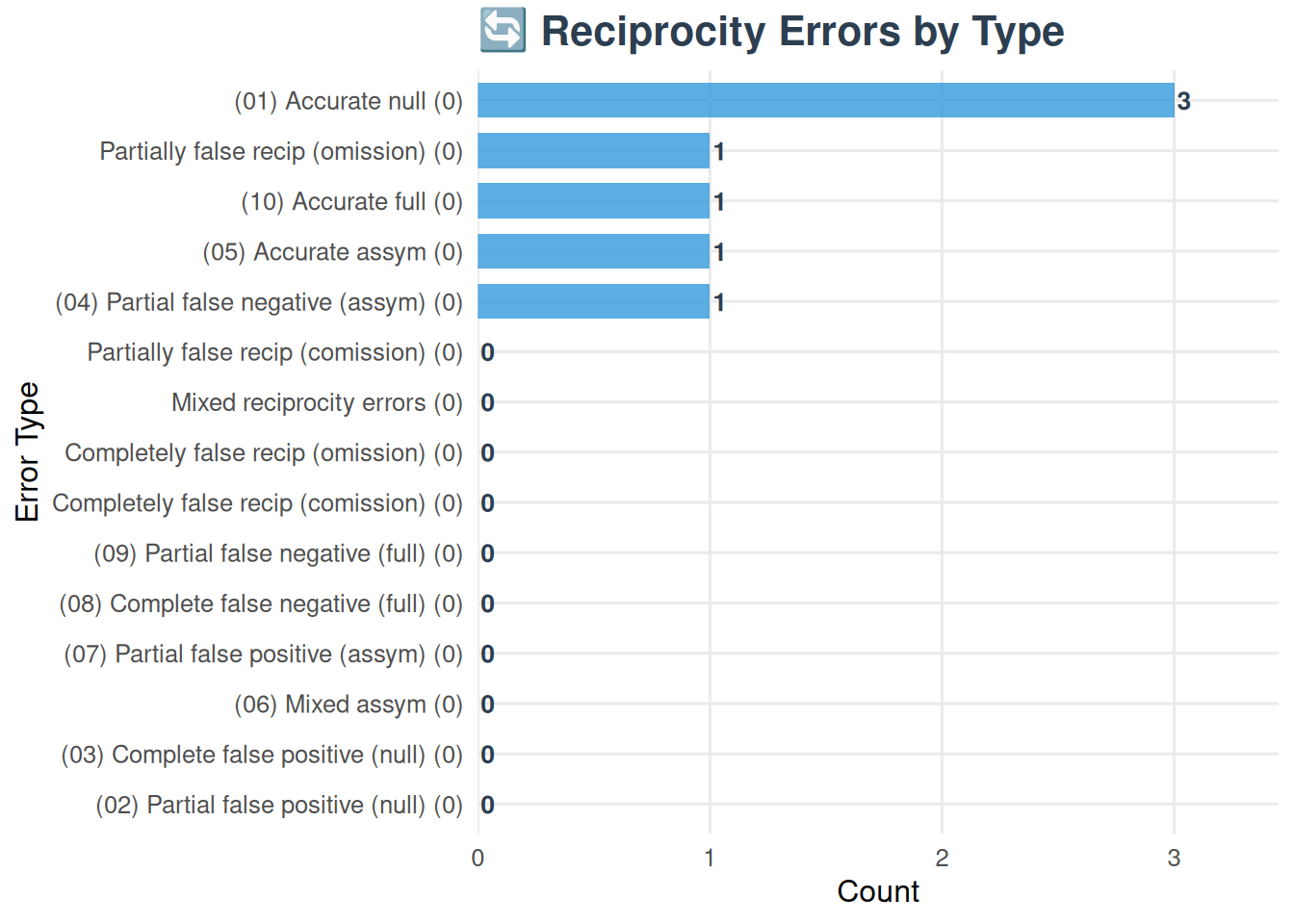
  filter(grepl("^\\([0-9]", name)) |>
  mutate(error_type = case_when(
    grepl("Accurate null", name) ~ "Accurate Null",
    grepl("Partial false positive \\(null\\)", name) ~ "Partial FP (Null)",
    grepl("Complete false positive \\(null\\)", name) ~ "Complete FP (Null)",
    grepl("Partial false negative \\(assym\\)", name) ~ "Partial FN (Asymm)",
    grepl("Accurate assym", name) ~ "Accurate Asymm",
    grepl("Mixed assym", name) ~ "Mixed Asymm",
    grepl("Partial false positive \\(assym\\)", name) ~ "Partial FP (Asymm)",
    grepl("Complete false negative \\(full\\)", name) ~ "Complete FN (Full)",
    grepl("Partial false negative \\(full\\)", name) ~ "Partial FN (Full)",
    grepl("Accurate full", name) ~ "Accurate Full",
    TRUE ~ "Other"
  ))

error_colors <- c("Accurate Null" = "#27ae60", "Accurate Asymm" = "#2ecc71", 
                  "Accurate Full" = "#16a085", "Partial FP (Null)" = "#f39c12",
                  "Partial FN (Asymm)" = "#e67e22", "Partial FN (Full)" = "#d35400",
                  "Complete FP (Null)" = "#e74c3c", "Complete FN (Full)" = "#c0392b",
                  "Partial FP (Asymm)" = "#8e44ad", "Mixed Asymm" = "#9b59b6", "Other" = "#95a5a6")

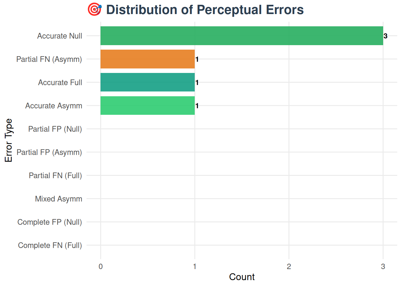
ggplot(census_summary, aes(x = reorder(error_type, value), y = value)) +
  geom_col(aes(fill = error_type), alpha = 0.9, width = 0.8) +
  geom_text(aes(label = ifelse(value > 0, value, "")), hjust = -0.1, size = 3.2, fontface = "bold") +
  scale_fill_manual(values = error_colors) + coord_flip() +
  labs(title = "🎯 Distribution of Perceptual Errors", x = "Error Type", y = "Count") +
  guides(fill = "none")

Individual Accuracy Analysis

Breaking down accuracy into four key measures: ego vs alter relationships, true positives vs negatives.

accuracy <- tie_level_accuracy(graph)
accuracy_df <- accuracy[, names(accuracy)]
class(accuracy_df) <- "data.frame"

accuracy_long <- accuracy_df |>
  select(-k) |>
  tidyr::pivot_longer(everything(), names_to = "measure", values_to = "probability") |>
  mutate(measure_clean = case_when(
    measure == "p_0_ego" ~ "True Negative (Ego)",
    measure == "p_1_ego" ~ "True Positive (Ego)", 
    measure == "p_0_alter" ~ "True Negative (Alter)",
    measure == "p_1_alter" ~ "True Positive (Alter)"
  ))

accuracy_colors <- c("True Negative (Ego)" = "#3498db", "True Positive (Ego)" = "#2980b9",
                     "True Negative (Alter)" = "#e74c3c", "True Positive (Alter)" = "#c0392b")

ggplot(accuracy_long, aes(x = measure_clean, y = probability)) +
  geom_violin(aes(fill = measure_clean), alpha = 0.7, trim = FALSE) +
  geom_boxplot(width = 0.2, alpha = 0.8) +
  geom_jitter(width = 0.15, alpha = 0.6, size = 2, color = "#2c3e50") +
  scale_fill_manual(values = accuracy_colors) +
  scale_y_continuous(labels = scales::percent_format()) +
  labs(title = "🎯 Individual-Level Accuracy Rates", x = "Accuracy Measure", y = "Accuracy Rate (%)") +
  guides(fill = "none") + theme(axis.text.x = element_text(angle = 30, hjust = 1))

Warning: Groups with fewer than two datapoints have been dropped.
ℹ Set `drop = FALSE` to consider such groups for position adjustment purposes.
Groups with fewer than two datapoints have been dropped.
ℹ Set `drop = FALSE` to consider such groups for position adjustment purposes.
Groups with fewer than two datapoints have been dropped.
ℹ Set `drop = FALSE` to consider such groups for position adjustment purposes.
Groups with fewer than two datapoints have been dropped.
ℹ Set `drop = FALSE` to consider such groups for position adjustment purposes.

Warning in max(data$density, na.rm = TRUE): no non-missing arguments to max;
returning -Inf

Warning: Computation failed in `stat_ydensity()`.
Caused by error in `$<-.data.frame`:
! replacement has 1 row, data has 0

Null Models and Statistical Testing

Generate realistic null distributions using individual accuracy rates.

# Sample networks and generate null distribution
set.seed(123)
sampled_networks <- sample_css_network(graph, keep_baseline = TRUE)
n_samples <- 100

null_samples <- replicate(n_samples, {
  sample_css_network(graph, keep_baseline = FALSE)
}, simplify = FALSE)

null_densities <- sapply(null_samples, function(nets) {
  if (length(nets) > 0) sum(nets[[1]]) / (4 * 3) else 0
})

observed_density <- sum(sampled_networks[[2]]) / (4 * 3)
p_value <- mean(null_densities >= observed_density)

# Visualization
ggplot(data.frame(density = null_densities), aes(x = density)) +
  geom_histogram(bins = 25, alpha = 0.8, fill = css_colors["primary"], color = "white") +
  geom_vline(xintercept = observed_density, color = css_colors["secondary"], linetype = "dashed", size = 1.2) +
  annotate("label", x = observed_density + 0.02, y = Inf, 
           label = paste("Observed\n", round(observed_density, 3)), vjust = 1.2, hjust = 0,
           color = css_colors["secondary"], fill = "white", fontface = "bold") +
  scale_x_continuous(labels = scales::percent_format()) +
  labs(title = "📊 Null Distribution of Network Density", 
       x = "Network Density (%)", y = "Frequency",
       caption = paste("P-value:", round(p_value, 4), "| Based on", n_samples, "null samples"))

Warning: Using `size` aesthetic for lines was deprecated in ggplot2 3.4.0.
ℹ Please use `linewidth` instead.

Key Insights

• Reciprocity Errors: Quantify how people misperceive mutual relationships
• Imaginary Census: 10-category taxonomy of all possible perceptual errors
• Individual Accuracy: Separate measures for ego/alter and positive/negative accuracy
• Null Models: Use individual accuracy rates to generate realistic chance distributions

---

Analysis with imaginarycss version 0.1.0