These functions can be used to generate null distributions for testing the prevalence of imaginary CSS. The null is a function of the individual level accuracy rates, in other words. Pr(i perceives a one| there is a one) and Pr(i perceives a zero| there is a zero).
Usage
tie_level_accuracy(graph, which_nets = NULL)

sample_css_network(
  graph,
  prob = tie_level_accuracy(graph),
  i = 1L:attr(graph, "netsize"),
  keep_baseline = TRUE
)
Arguments
- graph
A barry_graph object.
- which_nets
Integer vector. The networks to sample from.
- prob
A numeric vector of length 4L or a data frame (see details).
- i
Integer vector. The network to sample from.
- keep_baseline
Logical scalar. When
TRUE, the function returns the baseline network as the first element of the list.
Value
The function tie_level_accuracy returns a data frame with the following columns:
k: The perceiver id.p_0_ego: The probability of no tie between the perceiver (ego) and an alter.p_1_ego: The probability of a tie between the perceiver and an alter.p_0_alter: The probability of no tie between two alters.p_1_alter: The probability of a tie between two alters.
The function sample_css_network returns a list of square matrices of size
attr(graph, "netsize"). If keep_baseline = TRUE, the first element of
the list is the baseline network. Otherwise, it is not returned.
Details
There are two special cases worth mentioning. First, when the dyads in
question are all present the probability of true negative is set to NA.
On the other hand, if the dyads in question are all null, the probability of
true positive is NA as well. This doesn't affect the sample_css_network
function because those probabilities are unsed since tie/no tie probabilities
are according to the baseline graph, meaning that, for instance, a fully
connected network will never use the p_0_ego and p_0_alter
probabilities and an empty network will never use the p_1_ego and
p_1_alter probabilities.
The function sample_css_network samples perceived networks from the
baseline network. The baseline network is the first network in the
graph object. The function tie_level_accuracy can be used to
generate the probability vector.
The probability vector is a numeric vector of length 4L. The first
two elements are the probability of a tie/no tie between an ego and an alter.
The third and fourth elements are the probability of a tie/no tie between
two alters. When prob is a data frame, the function will sample from
each row of the data frame (returned from the function tie_level_accuracy).
Examples
# Using the Krackhardt advice network
data(krackhardt_advice)
data(krackhardt_advice_perceptions)
n_people <- 21
advice_matrix <- matrix(0L, nrow = n_people, ncol = n_people)
advice_matrix[cbind(krackhardt_advice$from, krackhardt_advice$to)] <-
krackhardt_advice$value
krack_graph <- new_barry_graph(
c(list(advice_matrix), krackhardt_advice_perceptions)
)
# Calculate accuracy rates
accuracy <- tie_level_accuracy(krack_graph)
print(accuracy)
#> k p_0_ego p_1_ego p_0_alter p_1_alter
#> 1 1 0.7619048 0.5263158 0.8086124 0.7251462
#> 2 2 0.5789474 0.7619048 0.8246445 0.7514793
#> 3 3 0.9000000 0.7000000 0.8190476 0.7235294
#> 4 4 0.9500000 0.7000000 0.7809524 0.6823529
#> 5 5 0.8000000 0.6000000 0.8142857 0.6588235
#> 6 6 0.7586207 0.8181818 0.7860697 0.6703911
#> 7 7 1.0000000 0.7142857 0.8199052 0.6863905
#> 8 8 0.7727273 0.6666667 0.7692308 0.6686047
#> 9 9 0.9130435 0.8235294 0.8502415 0.6994220
#> 10 10 0.7647059 0.8260870 0.7981221 0.7065868
#> 11 11 0.6923077 0.6428571 0.7892157 0.6875000
#> 12 12 0.8387097 0.6666667 0.7587940 0.6795580
#> 13 13 0.9000000 0.5000000 0.7900000 0.7277778
#> 14 14 0.8076923 0.7142857 0.7696078 0.7556818
#> 15 15 0.8125000 0.7500000 0.7757009 0.6867470
#> 16 16 0.8214286 0.7500000 0.7920792 0.6516854
#> 17 17 0.9230769 0.7142857 0.7941176 0.7500000
#> 18 18 0.6250000 0.7187500 0.8018018 0.7215190
#> 19 19 0.6000000 0.5333333 0.8000000 0.6342857
#> 20 20 0.9000000 0.6500000 0.7476190 0.7764706
#> 21 21 0.5714286 0.8076923 0.7916667 0.6768293
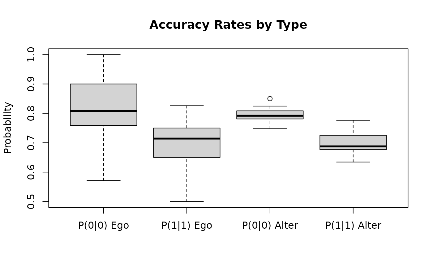
# Visualize accuracy patterns
boxplot(accuracy[, -1],
main = "Accuracy Rates by Type",
ylab = "Probability",
names = c("P(0|0) Ego", "P(1|1) Ego",
"P(0|0) Alter", "P(1|1) Alter"))
 # Using the Krackhardt advice network
data(krackhardt_advice)
data(krackhardt_advice_perceptions)
n_people <- 21
advice_matrix <- matrix(0L, nrow = n_people, ncol = n_people)
advice_matrix[cbind(krackhardt_advice$from, krackhardt_advice$to)] <-
krackhardt_advice$value
krack_graph <- new_barry_graph(
c(list(advice_matrix), krackhardt_advice_perceptions)
)
# Method 1: Using accuracy data frame (recommended)
accuracy <- tie_level_accuracy(krack_graph)
sampled_networks <- sample_css_network(krack_graph, prob = accuracy)
length(sampled_networks)
#> [1] 22
# Method 2: Using manual probability vector for a single perceiver
# p_0_ego, p_1_ego, p_0_alter, p_1_alter
manual_probs <- c(0.8, 0.9, 0.85, 0.75)
sampled_manual <- sample_css_network(
krack_graph,
prob = manual_probs,
i = 1,
keep_baseline = FALSE
)
# Using the Krackhardt advice network
data(krackhardt_advice)
data(krackhardt_advice_perceptions)
n_people <- 21
advice_matrix <- matrix(0L, nrow = n_people, ncol = n_people)
advice_matrix[cbind(krackhardt_advice$from, krackhardt_advice$to)] <-
krackhardt_advice$value
krack_graph <- new_barry_graph(
c(list(advice_matrix), krackhardt_advice_perceptions)
)
# Method 1: Using accuracy data frame (recommended)
accuracy <- tie_level_accuracy(krack_graph)
sampled_networks <- sample_css_network(krack_graph, prob = accuracy)
length(sampled_networks)
#> [1] 22
# Method 2: Using manual probability vector for a single perceiver
# p_0_ego, p_1_ego, p_0_alter, p_1_alter
manual_probs <- c(0.8, 0.9, 0.85, 0.75)
sampled_manual <- sample_css_network(
krack_graph,
prob = manual_probs,
i = 1,
keep_baseline = FALSE
)