library(imaginarycss)

# Load Krackhardt data
data(krackhardt_advice)
data(krackhardt_friendship)
data(krackhardt_friendship_perceptions)
data(krackhardt_advice_perceptions)

# Convert edge-list data frames to adjacency matrices
df_to_adjmat <- function(df) {
  n <- max(c(df$from, df$to))
  m <- matrix(0L, nrow = n, ncol = n)
  m[cbind(df$from, df$to)] <- df$value
  m
}

advice_matrix     <- df_to_adjmat(krackhardt_advice)
friendship_matrix <- df_to_adjmat(krackhardt_friendship)Imaginary Network Motifs: Testing Systematic Perception Errors
People do not perceive social networks randomly—their errors follow systematic patterns (Tanaka & Vega Yon, 2023). This vignette demonstrates how to use imaginarycss to (1) compute observed imaginary-census motif counts, (2) generate a null distribution that preserves each perceiver’s tie-level accuracy, and (3) test which motif patterns are significantly elevated or reduced relative to chance.
Setup
Data Overview
n <- nrow(advice_matrix)

# Network summary
data.frame(
  Network    = c("Friendship", "Advice"),
  Edges      = c(sum(friendship_matrix), sum(advice_matrix)),
  Density    = round(c(
    sum(friendship_matrix) / (n * (n - 1)),
    sum(advice_matrix)     / (n * (n - 1))
  ), 3)
)
Network Edges Density
1 Friendship 102 0.243
2 Advice 190 0.452Creating the CSS Graphs
Each graph bundles the true network (first element) with every individual’s perception.
friendship_graph <- new_barry_graph(
  c(list(friendship_matrix), krackhardt_friendship_perceptions)
)
advice_graph <- new_barry_graph(
  c(list(advice_matrix), krackhardt_advice_perceptions)
)
Observed Motif Counts
The imaginary census classifies every perceiver–dyad pair into one of ten categories. The summary() method aggregates counts across perceivers.
friendship_observed <- count_imaginary_census(friendship_graph)
advice_observed     <- count_imaginary_census(advice_graph)

# Friendship motifs (top 6)
head(summary(friendship_observed))
Accurate null Accurate assym
2472 529
Partial false positive (assym) Partial false positive (null)
378 276
Accurate full Partial false negative (full)
269 181 Accurate assym Accurate null
1052 992
Accurate full Partial false negative (assym)
469 463
Partial false positive (assym) Partial false negative (full)
412 395 Null-Model Testing
The test_imaginary_census() function generates null CSS samples for each network. Each sample preserves every perceiver’s four accuracy rates (true-positive/true-negative for ego/alter dyads) but randomises which specific dyads are misperceived. It then computes z-scores and two-sided empirical p-values.
set.seed(331)
friendship_test <- test_imaginary_census(friendship_graph, n_sim = 100)
advice_test     <- test_imaginary_census(advice_graph, n_sim = 100)
Results
The plot() method for imaginarycss_test objects shows a horizontal barplot of z-scores for each motif. Motifs whose z-score exceeds the critical threshold (dashed red lines) are coloured steelblue; those within the expected range under the null model are shown in grey.
# Print significant motifs
friendship_test
Imaginary-census significance test
Simulations: 100 | Alpha: 0.05
Significant motifs:
motif observed z_score p_value
Partial false positive (assym) 378 26.95 0
Accurate assym 529 -15.55 0
Accurate null 2472 14.57 0
Partial false positive (null) 276 -13.56 0
Mixed assym 98 13.30 0
Partial false negative (assym) 171 -5.64 0
Complete false positive (null) 3 -5.36 0
advice_testImaginary-census significance test
Simulations: 100 | Alpha: 0.05
Significant motifs:
motif observed z_score p_value
Partial false positive (assym) 412 7.87 0
Accurate null 992 7.38 0
Partial false positive (null) 343 -6.12 0
Accurate assym 1052 -5.33 0
Mixed assym 173 3.59 0
Complete false positive (null) 30 -3.58 0
# Visualise z-scores
plot(friendship_test, main = "Friendship: Motif Z-Scores vs Null")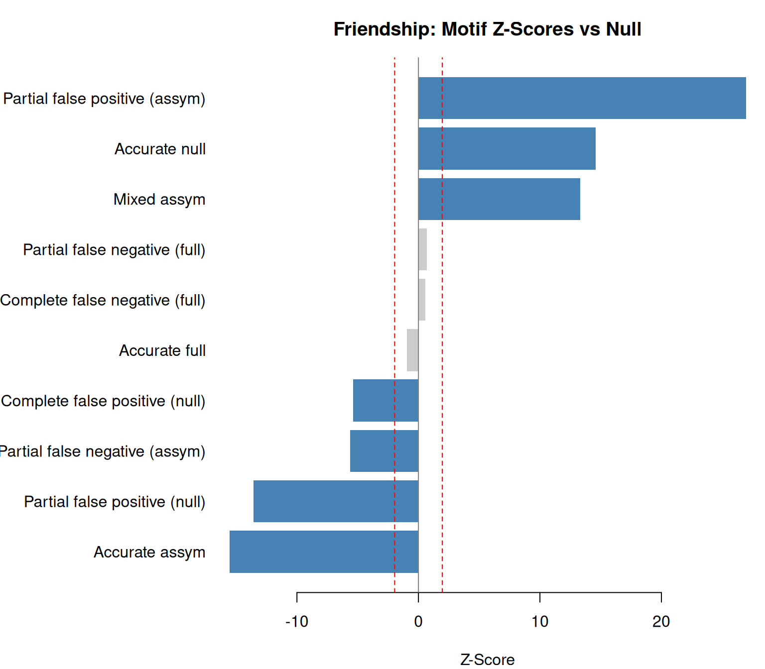
plot(advice_test, main = "Advice: Motif Z-Scores vs Null")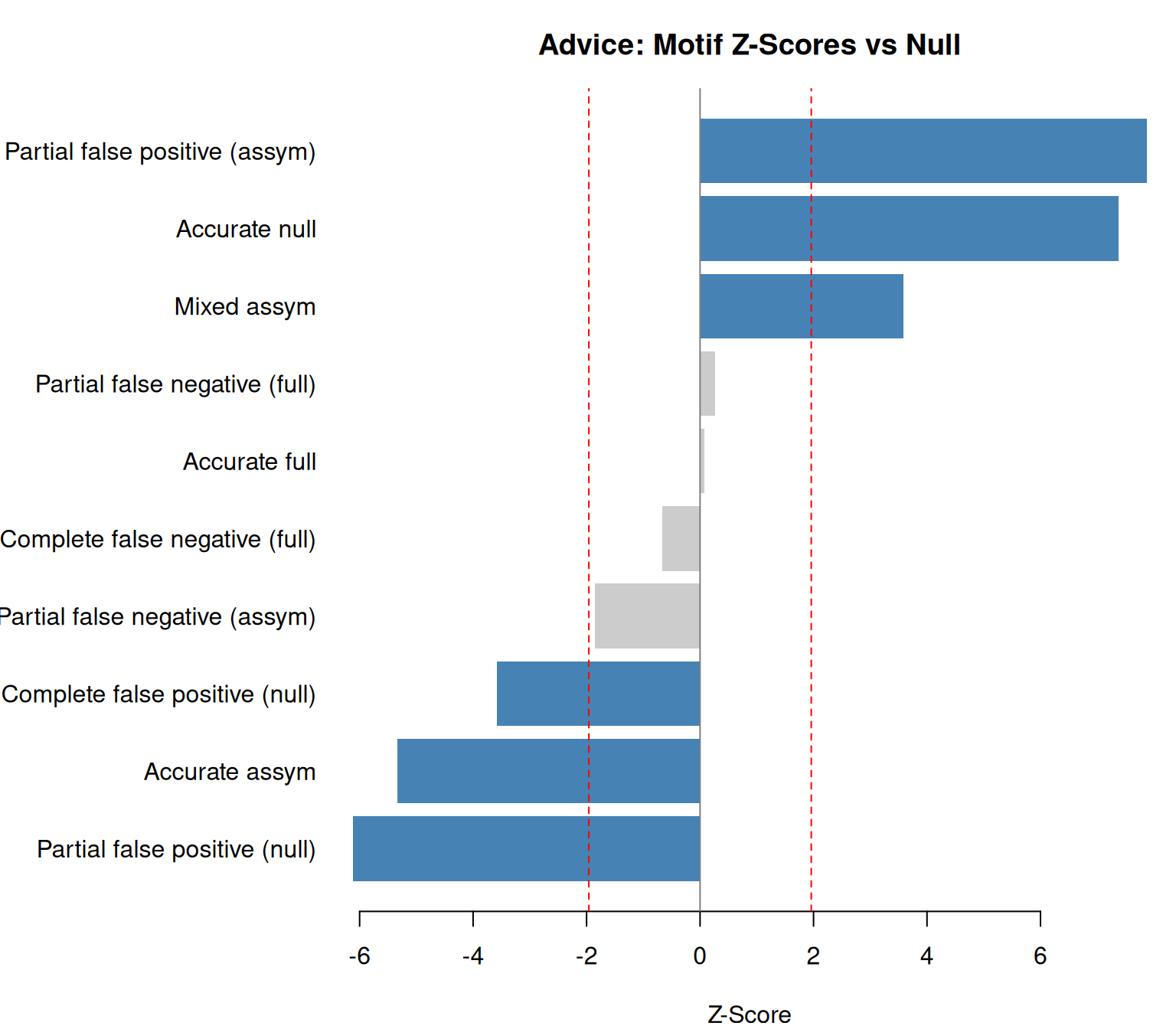
Full Summary
The summary() method shows all motifs with their test statistics.
summary(friendship_test)Imaginary-census significance test
Simulations: 100 | Alpha: 0.05
Motifs tested: 10 | Significant: 7
motif observed null_mean null_sd z_score p_value
Partial false positive (assym) 378 104.6 10.15 26.95 0.00
Accurate assym 529 790.0 16.78 -15.55 0.00
Accurate null 2472 2167.7 20.89 14.57 0.00
Partial false positive (null) 276 546.3 19.94 -13.56 0.00
Mixed assym 98 33.3 4.86 13.30 0.00
Partial false negative (assym) 171 248.0 13.65 -5.64 0.00
Complete false positive (null) 3 37.0 6.34 -5.36 0.00
Accurate full 269 278.6 10.07 -0.95 0.34
Partial false negative (full) 181 174.5 9.36 0.69 0.46
Complete false negative (full) 33 29.9 5.46 0.57 0.62
significant
TRUE
TRUE
TRUE
TRUE
TRUE
TRUE
TRUE
FALSE
FALSE
FALSETie-Level Accuracy
friendship_acc <- tie_level_accuracy(friendship_graph)
advice_acc     <- tie_level_accuracy(advice_graph)

# Mean individual accuracy
data.frame(
  Network = c("Friendship", "Advice"),
  TP      = round(c(
    mean(friendship_acc$p_1_ego, na.rm = TRUE),
    mean(advice_acc$p_1_ego,     na.rm = TRUE)
  ), 3),
  TN      = round(c(
    mean(friendship_acc$p_0_ego, na.rm = TRUE),
    mean(advice_acc$p_0_ego,     na.rm = TRUE)
  ), 3)
)
Network TP TN
1 Friendship 0.750 0.886
2 Advice 0.695 0.795Conclusion
By comparing observed motif counts against null distributions that preserve individual-level accuracy, the imaginary census reveals which perceptual errors are systematic rather than random. Elevated motifs indicate cognitive schemas (e.g., balance, reciprocity) that distort network perception beyond what individual accuracy rates alone would predict.