Krackhardt Advice Network
This vignette demonstrates a complete imaginarycss workflow using the classic Krackhardt (1987) dataset of 21 managers in a high-tech company. We construct a CSS object from the advice network and its individual perceptions, then compute accuracy rates and the imaginary census.
Data and Perceptions
The package ships the advice network as a data frame (krackhardt_advice) and a list of 21 perception matrices (krackhardt_advice_perceptions). We convert the edge-list to an adjacency matrix and bundle it with the perception data into a barry_graph object.
data(krackhardt_advice)
data(krackhardt_advice_perceptions)

# Convert edge-list data frame to adjacency matrix
n_people <- max(c(krackhardt_advice$from, krackhardt_advice$to))
advice_matrix <- matrix(0L, nrow = n_people, ncol = n_people)
advice_matrix[cbind(krackhardt_advice$from, krackhardt_advice$to)] <- krackhardt_advice$value

krack_graph <- new_barry_graph(c(list(advice_matrix), krackhardt_advice_perceptions))
We can see how the network looks (as an adjacency matrix):
print(krack_graph)A barry_graph with 22 networks of size 21
. . 1.00 . 1.00 . . . 1.00 . .
. . . . . 1.00 1.00 . . .
1.00 1.00 . 1.00 . 1.00 1.00 1.00 1.00 1.00
1.00 1.00 . . . 1.00 . 1.00 . 1.00
1.00 1.00 . . . 1.00 1.00 1.00 . 1.00
. . . . . . . . . .
. 1.00 . . . 1.00 . . . .
. 1.00 . 1.00 . 1.00 1.00 . . 1.00
1.00 1.00 . . . 1.00 1.00 1.00 . 1.00
1.00 1.00 1.00 1.00 1.00 . . 1.00 . .
Skipping 452 rows. Skipping 452 columns. Individual Accuracy
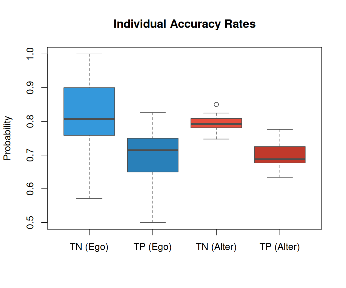
The function tie_level_accuracy() decomposes each perceiver’s accuracy into four probabilities, separating ego-involved from alter-only dyads and true positives from true negatives.
acc <- tie_level_accuracy(krack_graph)
acc
k p_0_ego p_1_ego p_0_alter p_1_alter
1 1 0.7619048 0.5263158 0.8086124 0.7251462
2 2 0.5789474 0.7619048 0.8246445 0.7514793
3 3 0.9000000 0.7000000 0.8190476 0.7235294
4 4 0.9500000 0.7000000 0.7809524 0.6823529
5 5 0.8000000 0.6000000 0.8142857 0.6588235
6 6 0.7586207 0.8181818 0.7860697 0.6703911
7 7 1.0000000 0.7142857 0.8199052 0.6863905
8 8 0.7727273 0.6666667 0.7692308 0.6686047
9 9 0.9130435 0.8235294 0.8502415 0.6994220
10 10 0.7647059 0.8260870 0.7981221 0.7065868
11 11 0.6923077 0.6428571 0.7892157 0.6875000
12 12 0.8387097 0.6666667 0.7587940 0.6795580
13 13 0.9000000 0.5000000 0.7900000 0.7277778
14 14 0.8076923 0.7142857 0.7696078 0.7556818
15 15 0.8125000 0.7500000 0.7757009 0.6867470
16 16 0.8214286 0.7500000 0.7920792 0.6516854
17 17 0.9230769 0.7142857 0.7941176 0.7500000
18 18 0.6250000 0.7187500 0.8018018 0.7215190
19 19 0.6000000 0.5333333 0.8000000 0.6342857
20 20 0.9000000 0.6500000 0.7476190 0.7764706
21 21 0.5714286 0.8076923 0.7916667 0.6768293We can further view this as a summary:
# Mean accuracy rates as a data.frame
data.frame(
  Measure = c("TP (Ego)", "TN (Ego)", "TP (Alter)", "TN (Alter)"),
  Mean    = round(c(
    mean(acc$p_1_ego,   na.rm = TRUE),
    mean(acc$p_0_ego,   na.rm = TRUE),
    mean(acc$p_1_alter, na.rm = TRUE),
    mean(acc$p_0_alter, na.rm = TRUE)
  ), 3)
)
Measure Mean
1 TP (Ego) 0.695
2 TN (Ego) 0.795
3 TP (Alter) 0.701
4 TN (Alter) 0.794
acc_mat <- as.matrix(acc[, c("p_0_ego", "p_1_ego", "p_0_alter", "p_1_alter")])
boxplot(
  acc_mat,
  names = c("TN (Ego)", "TP (Ego)", "TN (Alter)", "TP (Alter)"),
  ylab = "Probability",
  main = "Individual Accuracy Rates",
  col = c("#3498db", "#2980b9", "#e74c3c", "#c0392b"),
  border = "gray30"
)
Perceptual Structure
The imaginary census and reciprocity error counts summarize which types of misperception are most prevalent across all perceivers.
krack_census <- count_imaginary_census(krack_graph)
krack_recip  <- count_recip_errors(krack_graph)

# Top imaginary census motifs
head(krack_census, 5)
##   id                   name value
## 1  0 (01) Accurate null (0)    45
## 2  1 (01) Accurate null (1)    53
## 3  2 (01) Accurate null (2)    53
## 4  3 (01) Accurate null (3)    49
## 5  4 (01) Accurate null (4)    47

# Reciprocity errors
head(krack_recip, 5)
##   id                                 name value
## 1  0 Partially false recip (omission) (0)    46
## 2  1 Partially false recip (omission) (1)    31
## 3  2 Partially false recip (omission) (2)    37
## 4  3 Partially false recip (omission) (3)    40
## 5  4 Partially false recip (omission) (4)    52
Organizational Takeaways
We now consolidate key statistics from the analysis above. The summary table below reports network-level properties (size and density) alongside individual-level accuracy measures, identifying which managers perceive the advice network most and least accurately.
density <- sum(advice_matrix) / (n_people * (n_people - 1))
avg_tp  <- mean(acc$p_1_ego, na.rm = TRUE)
best    <- which.max(acc$p_1_ego)
worst   <- which.min(acc$p_1_ego)

# Network summary
data.frame(
  Statistic = c("Employees", "Advice network density",
                "Avg TP (Ego)", "Most accurate perceiver",
                "Least accurate perceiver"),
  Value     = c(n_people, round(density, 3), round(avg_tp, 3),
                paste0(best, " (", round(acc$p_1_ego[best], 3), ")"),
                paste0(worst, " (", round(acc$p_1_ego[worst], 3), ")"))
)
##                  Statistic      Value
## 1                Employees         21
## 2   Advice network density      0.452
## 3             Avg TP (Ego)      0.695
## 4  Most accurate perceiver 10 (0.826)
## 5 Least accurate perceiver   13 (0.5)
The advice network is relatively dense (45%), meaning nearly half of all possible ties exist. On average, managers correctly identify about 70% of existing ego-involved advice ties. Manager 10 stands out as the most perceptive, while Manager 13 shows the most room for improvement. These differences in perceptual accuracy may reflect variation in organizational position or engagement with the informal advice structure.